UPDATE March 31, 2024: There is no sign error. It was our own calculation error.
----
(x, y + dy) (x + dx, y + dy)
--------------------
| |
| |
| |
--------------------
(x, y) (x + dx, y)
Above, we have drawn a small rectangle according to the coordinates.

(Ruler and protractor photo pxhere.com)
The metric g determines the "proper" distances between coordinate points. By proper we mean things that someone living on the surface measures with a ruler and a protractor. If we measure proper distances around (x, y), we can draw cartesian coordinates X and Y, for which the metric G is almost the euclidian metric:
1 0
0 1.
The above rectangle in the coordinate plane X, Y looks something like this:
_______----______
\ /
\ /
\ /
-----___----
The rectangle is distorted and its sides are not straight lines.
This Wikipedia picture shows what happens to a longitude, latitude coordinate rectangle when we draw it in "more proper" coordinates X and Y. The lines are bulging outward.
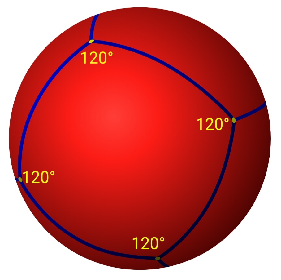
In the definition of Riemann curvature, the man does not walk along coordinate lines, but along geodesics which are the "straightest" possible paths in the metric. Geodesics minimize the distance between the endpoints of the line. For a sphere, the geodesics are the great circles.
We measure the proper angles at each corner of the path. If the angles add up to 360 degrees, it is a flat plane. If the angles add up to > 360 degrees, the curvature is positive. Why proper angles? Because that is the angle which the man sees at the corner. He is not interested in the coordinates which we happened to choose. The man in interested in things which he can measure.
We have to find the formula which determines the proper angles at the corners. That will be the correct Riemann tensor formula.
Geodesics and coordinate lines
^ y
| / f(x) geodesic
| /
| /
•----------------------> x coordinate line
Let us have a geodesic f which starts from a point P initially to the direction of the coordinate line x. The geodesic f diverts from the coordinate line.
The geodesic f differs from the coordinate line in two ways:
1. fy(x) tells us how much the geodesic has diverted to the y direction from the x coordinate line;
2. fx(x) tells us how much the proper distance measured along the geodesic differs from the proper distance measured along the x coordinate line.
The geodesic minimizes the proper distance between any two of its points. The variation where we slightly displace a part of the geodesic must always increase the proper distance measured along the geodesic.
Maybe we get a unique formula for f from the variational constraint?

If x and y are orthogonal in the metric g, then our diagram is concerned with
Γ²₁₁ = 1/2 * 1 / g₂₂ * -∂ g₁₁ / dy
and
Γ¹₁₁ = 1/2 * 1 / g₁₁ * ∂ g₁₁ / dx.
Does the Christoffel symbol reveal us the correct geodesic? People say that the above formula tells how much the basis vector of k turns or grows to the i direction if we move a short distance to the direction of l.
The Christoffel symbols consist of first derivatives. They cannot describe the gradual turning up of the geodesic f in the diagram. But they can describe the change in the metric g₁₁ as we walk along the x coordinate line. In the case of polar coordinates on a plane, Γ²₁₁ = 0 and Γ¹₁₁ = 0, which are correct descriptions of what would happen in the diagram in that case.
The formula of the covariant derivative
The function x maps the cartesian coordinate plane ℝ² to a curved surface. The basis vectors are defined:

Let

be a mapping from ℝ² to vectors of the tangent plane at the image of the point in ℝ². Let

be another mapping. The covariant derivative of u along v is defined:

When calculating the "difference" of u at a location P and at a slightly displaced location Q, we need a way to transport the old value of u in the tangent plane of P to the tangent plane of Q. The Levi-Civita connection is supposed to do this transport in a "natural" way.
This reminds us of our vector transport problem. How to transport a vector in a "natural" way from P to Q?
The Levi-Civita connection
We say that a vector field X is a parallel transport of the vector ξ along the curve γ, iff

The connection ∇ above measures how much the vector X "changes" when we walk along the curve γ. The vector X is not allowed to change at all.

The connection which we use is the Levi-Civita connection. In the coordinate form,
∇X Y
is defined as:


Let X be the tangent vectors of a path γ. If the vector field Y describes the parallel transport of a vector along the path, then ∇X Y should be zero everywhere on the path. The numerical value is calculated from the metric using the Christoffel symbol formula. According to Wikipedia, the definition is essentially due to Elwin Bruno Christoffel in the year 1869.
A method to determine the rotation of a transported vector
Now we realize that there might be a relatively simple way to determine the amount of rotation in a loop.
orthogonal coordinate lines
---/--/--|--\--\--- coordinate line
If orthogonal coordinate lines "fan out" like in the diagram above, then the coordinate line is not a geodesic. A transported vector will turn according to how much the lines fan out?
The calculation may be complicated by the fact that the coordinate line may be curvy to many directions?
^
/
/
-------->
Also, the coordinates may be skewed.
Transport of a radial vector on a sphere along a coordinate line loop
We use on the spherical surface the metric and the r and φ coordinates of the previous blog post.
Let Y be a vector which everywhere points along the r axis, to the origin. The length of Y is constant in the r coordinate, but not in the proper length.
We choose the path γ as a small loop along coordinate lines of r and φ. On Earth that would mean a coordinate rectangle along meridians and latitude lines. The vector Y points everywhere along the meridian lines to the north.

(Picture by Hellerick
https://commons.m.wikimedia.org/wiki/File:Division_of_the_Earth_into_Gauss-Krueger_zones_-_Globe.svg )
walk around
---->
meridian line
-------------
| | latitude line
| |
------------- γ path (= X)
-----> Y
^ φ (coordinate 2)
|
------> r (coordinate 1)
The vector Y is not a parallel transported around γ, because the latitude coordinate lines are not great circles. The meridians are great circles, and along them, Y is parallel transported.
Using the idea of the preceding section, the meridian coordinate lines "fan out" when we walk along a latitude line. The fanning is stronger close to the North Pole than close to the equator.
In the formula

the derivative ∂j is zero because Y is constant. The terms with the Christoffel symbols Γ should tell us how much Y differs from a parallel transport. The difference tells us how much a parallel transported vector would have turned relative to Y after completing the loop. The X in the formula is the tangents of the path: γ'(t).
The r coordinate lines (latitude lines) in the rectangle are not great circles. The formula should show that the constant vector Y turns relative to a parallel transport.
The Christoffel symbol terms should recognize that we are not walking around a great circle, and calculate how much we divert from it.
The proper angle at each corner of the rectangle is 90 degrees. If the latitude lines were geodesics ("straight lines"), we would obtain a result that the rectangle is in a flat geometry: the sum of corner proper angles is 360 degrees. But it is on a surface of a sphere. The latitude lines are closer to the center of the rectangle than the corresponding great circle lines would be. That is, the latitude lines "curve inward".
Let us then analyze what the connection formula calculates when we walk along a latitude line.
1. X² differs from zero and X¹ is zero.
2. Y¹ differs from zero and Y² is zero.
3. In the formula, j = 2 and k = 1.
4. What is Γ¹₂₁ ∂₁ ? The coordinate vector ∂₁ points to the r direction (along a meridian). We have
Γ¹₂₁ = 1/2 * 1 / g₁₁ * ∂₂ g₁₁ = 0.
5. What is Γ²₂₂ ∂₂ ?
Γ²₂₂ = 1/2 * 1 / g₂₂ * ∂₂ g₂₂ = 0.
The connection should be zero when we walk along r (meridian). But why it is zero along φ (latitude)?
Conclusions
The sign error was our own calculation error. Wikipedia was right.
No comments:
Post a Comment